Site Example 1: Manistee Lake Sediment Toxicity EDA
The overall project goals were:
• Review available data on the sediments in Manistee Lake. Evaluate these data using EDA to develop a conceptual site model (CSM) to help understand the contaminant issues in the lake.
• Develop an “inventory and action plan” that assessed the major sources of industrial pollution, major sediment pollutants of concern, and propose courses of action.
• Create a presentation to increase local awareness and start discussions.
• Evaluate and design a plan for further sampling.
Manistee Lake Setting and Historical Impacts
The Manistee watershed encompasses more than 5000 square kilometers, 1930 square miles. The lake is a drowned river mouth, fed by the Manistee River from the NE and the Little Manistee River from the SE. A channel connects the lake to Lake Michigan. Flow is generally SE to NW with crossflow across the northern portion from the Manistee River west to Lake Michigan. The lake has an area of about 930 square acres and a maximum depth of about 50 feet. Manistee Lake was once a large bay of Lake Michigan; water levels dropped and they became separated by sand bars and low dunes.
The history of Manistee Lake includes more than a century and a half of industrial usage. Contamination of the lake bottom sediments is extensive, resulting in the near elimination of the natural populations of benthic organisms and creating a negative impact on the lake at all trophic levels.
Study Background
Sediment contaminants were quantified in Manistee Lake at 14 sampling locations (Figure 1) in a study by Rediske et al. (2001). EDA was used to discern whether additional insights could be gained from the data for better understanding of the lake’s environment.
Approach
EDA focused initially on metals and metalloids, total organic carbon (TOC), and hexane extractable materials with regard to descriptive statistics, depths in the sediments, concentrations, and sampling locations. Further evaluation added additional contaminants and potential pollutant sources. Benthic organism % mortality and counts were evaluated within this context, with an emphasis on identifying correlations between organism mortality, individual or multiple contaminants, and industrial activities that might be the contaminant source.
EDA of the chemicals versus four organism studies used stepwise multiple regression analysis and the most likely chemical causes of organism mortality were identified. The inventory of industrial activity in the lake vicinity and scoring of these activities for the “significant contamination factors,” (i.e., contaminants from the stepwise regression analysis that most impacted the organisms) was done. Results were plotted versus location along the lake with the highest scoring industrial activities highlighted. A CSM for sediment organism mortality was the result.
Results
The first analysis was to determine whether any of the constituents determined in the sediments were found preferentially at any particular depth(s) in the sediments. This was done by creating both dotplots and box and whisker plots of each of the constituents versus depth level. Figure 2 displays, as an example, such a box and whiskers plot for mercury (modified by assigning the reporting limit to samples reported at less than that limit, i.e., a conservative approach). The depth level S is for surface samples acquired using a Ponar sediment sampler whereas T, M, and B refer to top, middle and bottom core sections, respectively.
Boxplots have five components; more rigorous definitions of which can be found in Velleman. These are:
• The outlined central box depicts the middle half of the data between the 25th and the 75th percentiles.
• The horizontal line across the box marks the median.
• The whiskers extend from the top and bottom of the box to depict the extent of the main body of the data.
• In addition, extreme data values are plotted individually, usually with a circle.
• Very extreme values are plotted with a starburst.
In addition to these components the 95% confidence intervals of the data can be depicted with a shaded area. If the shaded areas for two or more groups do not overlap then there is 95% statistical confidence that their medians are different. Using such plots it was possible to observe that, in general, the contaminants of concern were primarily found in the uppermost lake sediments (Figure 2, S and T), potentially indicating anthropogenic origin.
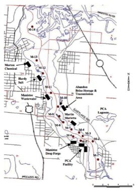
Figure 1. Manistee Sampling Locations from Rediske et al.
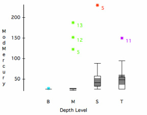
Figure 2. Box and Whiskers Plot for Mercury
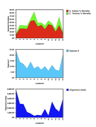
Figure 3. Organism Area Plots vs. Sampling Location
Rediske et al. performed two types of biological studies. One of these consisted of counting organisms in the collected sediment samples at each location. A value was assigned to the total number of organisms counted for each location and the species were noted and counted. This resulted in two biological values for each surface sampling location that were used in this EDA:
- 1. Organisms (total), and
- 2. Species #
The second type of biological study was independent laboratory tests of acute toxicity, via exposure to the actual sediments collected at each location, for two types of organisms. The organisms were:
- 1. Hyalella Azteca (amphipod), and
- 2. Chironomus Tentans (midge)
Eight replicate toxicity tests were done with each organism for each location. For the EDA the final average number surviving at each location was converted to a percent mortality value.
Boxplots of the organism studies indicated that the sediment control location mortalities (Figure 1, M-1 and M-14) were very different from the others along the length of the lake. By the time one arrives at Locations M-2 and M-13, organism mortality/disappearance is worsened by a range of factors from 1.6 to 5.5. This indicates significant sediment toxicity in the industrialized areas of the lake.
Area charts of the four sets of biological study results are displayed versus sampling location in Figure 3.
The charts for sediment mortality to H. Azteca and C. Tentans are stacked (Figure 3, top), whereas the magnitudes of the values for Species # and Organisms (Total) were too different for stacking without applying a data transformation. The percent mortality of the two organisms track one another very well and appear to be almost perfect counterparts to the organism and species # counts, with increased percent mortality corresponding very closely with reductions in the numbers and species of organisms natively present in the sediments. These plots illustrate the extreme toxicity of the shallow Manistee Lake sediments just beyond the river mouths (i.e., the control locations) within the lake.
Accounting for the specific environmental factors that contribute to the sudden increase in organism mortality upon entering the lake environment is important for a variety of reasons, including:
- 1. The levels of these toxic chemicals need to be reduced to increase biodiversity
- 2. Identifying the primary contaminants of concern might also identify the sources, creating an opportunity to control their discharge
- 3. Predictions of residence time and fate in the sediments might be possible based on the contaminant chemistry and the geochemistry
- 4. Additional sampling with increased focus on the most toxic areas can be planned
- 5. A conceptual model of the lake bed and its environment can begin to be developed.
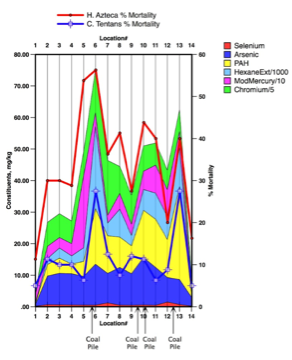
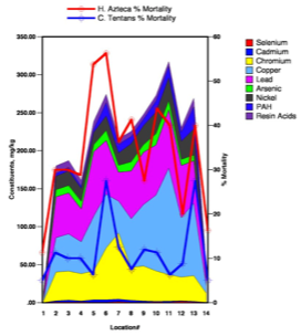
The next part of the EDA plotted the results of these organism studies versus their position along the lake. Figure 4 illustrates the complexity of understanding the specifics of toxicity to these organisms by also depicting stacked area charts of a variety of selected contaminant concentrations.
Virtually every measured contaminant in these surface sediment (Ponar) samples increased dramatically in concentration beyond the river mouth locations (control Locations 1 and 14) within the lake (Locations 2 through 13). The Percent Mortality lines for H. Azteca and C. Tentans overlying these area graphs (Figure 4) show the extremely close correspondence between the most highly contaminated zones and the toxicity of the sediments to these organisms. Cumulative, rather than individual, toxic contaminant impacts might be implied by these charts, so that possibility was further evaluated.
To determine whether individual toxicities or combined contaminant impacts were responsible a stepwise multiple regression analysis was the next phase of this EDA. This was done using the program DataDesk to develop a “model” for the impacts of the various contaminants on the organisms. The familiar simple linear regression, y = mx+a, describes the relationship between a response variable such as mortality (y) and a predictor variable such as a contaminant concentration (x). The data are plotted as a scatterplot that shows the datapoints, a regression line (based on the regression equation where m = slope and a = y axis intercept), and confidence interval boundaries, usually set at 95% confidence for environmental studies. A multiple regression includes more than one predictor variable to try to further account for the response variable values. However, the results of a multiple regression become difficult to visualize. Using only two predictor variables the straight line of the simple regression becomes a flat surface. Further addition of predictors adds additional dimensions. Because of this, numerical values must be used to explain the model rather than figures.
To understand whether predictor variables (such as arsenic, lead, hexane extractables, etc.) are significant and predict response values (such as H. Azteca % Mortality, Species #, etc.) requires the interpretation of tables containing t-ratios, probabilities, and R2 fit values. A discussion of these values and their interpretation is beyond the scope of this blog but can be found in standard statistics textbooks and the references cited. In summary, the Pearson Product Moment Correlation values for the selected organism study, versus all the possible predictors, (contaminants) is developed. This yields the residual correlations used in the stepwise regression analysis. The predictor variables are then individually added stepwise (hence the name) to the regression model, each causing its own residual correlation to go to zero and generating a probability. Regression begins with the highest residual correlation. In the case of H. Azteca this was arsenic at 0.756 residual. Additional contaminant predictors were added to the regression until the t-ratio probability of the last added predictor was greater than 0.05, indicating that that contaminant was not significant to mortality of the organism at the 95% confidence level.
The results of the stepwise multiple regression analyses are provided in Table 1 (below).
The stepwise multiple regression analyses indicated that certain sediment contaminants were well correlated with the loss of organisms in Manistee Lake. These contaminants and their apparent order of importance were:
As > Cr, hexane extractables, PAH > Hg, Se
Following this modeling, facilities along the lake shoreline were “scored” with respect to industrial processes and on-site materials that might generate this particular suite of contaminants. The highest scores were associated with facilities that stored coal or coke in piles along the shoreline of the lake. Figure 5 depicts the locations of these coal storage piles versus these important sediment contaminants from the stepwise regression and plots these versus the organism mortality values.
The results indicate that coal contamination of the bottom sediments along the shoreline seems to exert a substantial negative impact on the benthic organisms in those areas and immediately downgradient from them.
Conclusions
Several important conclusions resulted from the EDA study of Manistee Lake. These were:
1. The contaminants of concern were primarily found in the uppermost lake sediments, indicative of anthropogenic origin.
2. Many contaminants increased in concentration along the flowpath.
3. Area plots of the results of the sediment organism studies versus sample locations showed very good correspondence among the four biological approaches.
4. Mortality/disappearance worsened by factors of 1.6 to 5.5 immediately within the lake relative to controls.
5. There was excellent correspondence between organism mortality and locations of very high total contamination concentrations.
6. Stepwise multiple regression analyses indicated that certain sediment contaminants were well correlated with the dearth of organisms in Lake Manistee.
EDA elucidated that facilities hosting coal/coke storage piles were most strongly associated with contaminant concentrations and organism mortality, establishing a major portion of a conceptual site model. The results illustrate where cleanup could be focused to increase the populations of benthic organisms in Manistee Lake and increase its biodiversity.
| Study | Significant Predictors |
Outlier Locations |
Model Fit(R2 value) | F-Ratio |
| H. Azteca % Mortality | As, Hg, Hexane Extractables, Se | 12 | 97.7% | 109 |
| C. Tentans % Mortality | Hexane Extractables, Cr | 13 (PAH) | 81.7% | 20.3 |
| Organisms (total) | As, Cr | 62.0% | 11.6 | |
| Species # | As | 12, 13 (PAH) | 88.0% | 32.8 |


