


This is Site Example 2 of PASS' series on using exploratory and inferential data analysis (EDA) to solve practical problems in complex scenarios. Part 1 introduced EDA. A completely different real-word usage is illustrated in Site Example 1.
Example 2: Big Z Corporation Litigation
This EDA resulted from a lawsuit for air and soil contamination where PASS's Robert Powell was an expert witness. Although a real circumstance, the specifics have been modified for client anonymity.
Big Z Corporation (Big Z), was sued by a regional authority (RA), accused of contaminating soils in the vicinity of Big Z with zinc (Zn) via air deposition over a period of years. The RA collected soil samples from numerous locations outside the boundaries of Big Z and had them analyzed for Zn and other metals. Because Big Z was assumed to be the largest Zn user in the area, the finding of high Zn concentrations in many of the soil samples was sufficient for the RA to blame Big Z.
As the soil chemistry expert Mr. Powell did EDA on the RA soil data to determine whether there was information sufficient to conclude that Big Z was the contamination source. The analyses presented are an important subset of the EDA that was done.
Approach
The soil data were subjected to a variety of comparative, statistical and mapping procedures. This was to assess whether the data pointed solely to Big Z as the source or whether other sources might be responsible. Other potential sources were natural soil mineralogy, historic activities, and other facilities. Initial procedures also included comparison of the soil concentrations to Michigan’s regulatory requirements, the Part 201 Residential and Commercial 1 Generic Cleanup Criteria and Screening Levels, and to those concentrations found by the Michigan Background Soil Survey 2005.
Statistical EDA procedures for the soil samples included simple descriptive statistics of individual contaminant concentrations (mean, median, range, skewness, etc.) along with spatial, trend and regression analyses to determine whether anything pointed to a source.
It was important to look at the industrial and urban Zn uses, because Big Z is in an area that has been highly industrialized for more than a century. The industrial and commercial activities that occurred within and surrounding that area were also investigated, to provide additional context for the EDA results. These preliminary investigations showed that Zn had been widely used and disseminated for about 150 years in the area and that the "natural" soil background was also higher than the average statewide Zn concentrations. The industrial fill materials historically used to level properties across the region were also high in all the relevant metals.
Sample concentration and location data were input into either a spreadsheet or the EDA program Aabel (Gigawiz.com) and transposed, coded or reorganized when necessary for the analyses. Most of the EDA analyses and statistical visualizations were done in Aabel, although certain of the data were also evaluated using the R statistical program and some confirmatory statistics were carried out using the program DataDesk.
To determine whether patterns of soil deposition would emerge in relation to potential sources, transects were developed along lines of samples to establish whether there was any directionality to the metals distribution.
To evaluate the transects analysis it was hypothesized:
Following the transect analyses, an analysis of spatial concentration “zones” with distance from the Big Z property boundaries was done. The hypotheses for this analysis were essentially the same as for the transect analyses but with a different spatial approach.
Example 2: Big Z Corporation Litigation
This EDA resulted from a lawsuit for air and soil contamination where PASS's Robert Powell was an expert witness. Although a real circumstance, the specifics have been modified for client anonymity.
Big Z Corporation (Big Z), was sued by a regional authority (RA), accused of contaminating soils in the vicinity of Big Z with zinc (Zn) via air deposition over a period of years. The RA collected soil samples from numerous locations outside the boundaries of Big Z and had them analyzed for Zn and other metals. Because Big Z was assumed to be the largest Zn user in the area, the finding of high Zn concentrations in many of the soil samples was sufficient for the RA to blame Big Z.
As the soil chemistry expert Mr. Powell did EDA on the RA soil data to determine whether there was information sufficient to conclude that Big Z was the contamination source. The analyses presented are an important subset of the EDA that was done.
Approach
The soil data were subjected to a variety of comparative, statistical and mapping procedures. This was to assess whether the data pointed solely to Big Z as the source or whether other sources might be responsible. Other potential sources were natural soil mineralogy, historic activities, and other facilities. Initial procedures also included comparison of the soil concentrations to Michigan’s regulatory requirements, the Part 201 Residential and Commercial 1 Generic Cleanup Criteria and Screening Levels, and to those concentrations found by the Michigan Background Soil Survey 2005.
Statistical EDA procedures for the soil samples included simple descriptive statistics of individual contaminant concentrations (mean, median, range, skewness, etc.) along with spatial, trend and regression analyses to determine whether anything pointed to a source.
It was important to look at the industrial and urban Zn uses, because Big Z is in an area that has been highly industrialized for more than a century. The industrial and commercial activities that occurred within and surrounding that area were also investigated, to provide additional context for the EDA results. These preliminary investigations showed that Zn had been widely used and disseminated for about 150 years in the area and that the "natural" soil background was also higher than the average statewide Zn concentrations. The industrial fill materials historically used to level properties across the region were also high in all the relevant metals.
Sample concentration and location data were input into either a spreadsheet or the EDA program Aabel (Gigawiz.com) and transposed, coded or reorganized when necessary for the analyses. Most of the EDA analyses and statistical visualizations were done in Aabel, although certain of the data were also evaluated using the R statistical program and some confirmatory statistics were carried out using the program DataDesk.
To determine whether patterns of soil deposition would emerge in relation to potential sources, transects were developed along lines of samples to establish whether there was any directionality to the metals distribution.
To evaluate the transects analysis it was hypothesized:
- 1. A positive likelihood of Big Z being the source could be shown by a general increase in Zn concentrations as transects of soil samples approached the Big Z property boundary (i.e., consistently increasing soil concentrations with approach to the facility); this result would require a plurality of transects showing this pattern.
- 2. A negative likelihood of Big Z being the source could be shown by decreases in, or randomness of, Zn concentrations as transects of soil samples approached the Big Z property boundary (i.e., decreasing or random soil concentrations with approach to the facility).
- 3. A pattern of high soil concentrations at a generally consistent distance along the transects from the Big Z property boundaries might imply Zn sourcing by the Big Z facility (maximum soil deposition at a fairly consistent distance from the facility).
- 4. A random relationship in soil Zn concentrations, with respect to Big Z boundaries, increases the likelihood of numerous, possibly localized, sources for the Zn.
Following the transect analyses, an analysis of spatial concentration “zones” with distance from the Big Z property boundaries was done. The hypotheses for this analysis were essentially the same as for the transect analyses but with a different spatial approach.

Figure 1. Sampling Locations, Transect Overview, and Zn Concentrations

Figure 2. A' - A Zinc Concentration Transect

Figure 3. Spatial Zones for Zinc Analysis
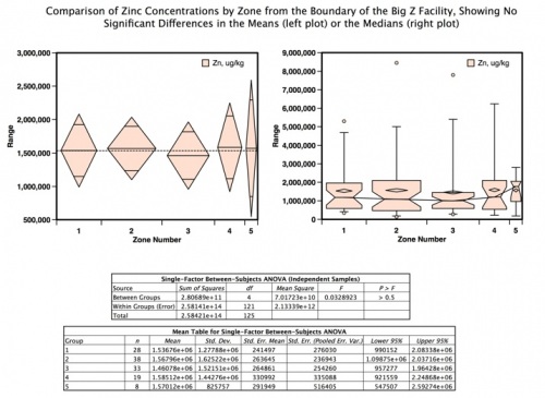
Figure 4. Comparisons of Zone Means and Medians for Zinc
Results
Figure 1 provides an overview for the transect analyses, showing Zn data in the vicinity of Big Z. This plot, created in the program Aabel, depicts:
• Big Z property boundaries (light blue area)
• Soil sample locations (all westerly of Big Z)
• Transects across the soil locations
• The general location of the Big Z operations
• Other potential stationary industrial emission sources (by facility code)
• Color-filled contours for the Zn concentrations to show areas of higher Zn concentration versus lower.
The transect overview in Figure 1 also displays information about sampling points that were high statistical lognormal outliers at the 95% upper confidence level for one or multiple metals (i.e., they were outside the expected concentration range based on the complete body of data at 95% confidence), which could potentially be called “hotspots,” highlighted by the type of marker:
• A small yellow-tan circle indicates no constituents were outliers relative to the body of the data at that sampling location.
• A circular red “beach-ball” marker indicates a sampling location was an outlier for a metal other than Zn.
• A hexagonal black marker indicates the sample location was an outlier only for Zn.
• A hexagonal red marker indicates that the sample location was an outlier for Zn and at least one of the other metals.
The transects in Figure 1 are shown as orange lines or polygons. The distal end (furthest away relative to the Big Z facility) of the transect line/polygon is labeled with a capital letter and a prime symbol ( ‘ ) and the proximal end (closest to Big Z) with just a plain capital letter; for example “A’ – A” signifies a transect. A total of nine transects were done on each dataset and labeled A’ – A through I’ – I. Each transect was subjected to regression analysis, i.e., Zn concentration versus distance from the Big Z property boundary as well as individual visualization using either bubble charts or spatial bar charts. An example is provided in Figure 2 for transect A’ – A.
Reviewing all the transect figures, such as Figure 2, showed that the r2 values were quite low, indicating that linear distance/direction along the transect line towards Big Z does not account well for the Zn concentrations. It is also observed that the slopes of the regression lines are generally not very large in either direction while scatter of the points about those lines is relatively large, supporting the r2 determinations and the general lack of trending in concentration versus distance from the Big Z property.
Table 2 summarizes the r2 and slope values for each transect and whether the slopes showed increasing Zn trends toward or away from the property. It shows that there were similar numbers of transects with slopes in either direction. This tends to support the dispersed random-appearing hotspots and colored contours of Figure 6. These results also support Hypotheses 2 and 4 (above), or randomness of Zn concentrations relative to the Big Z property boundaries and the likelihood of numerous localized Zn sources.
As an additional check on the spatial relationship of the Zn concentrations in the soil samples relative to the Big Z boundaries, the Zn data were separated into five spatially equivalent zones corresponding to surface areas replicated using the approximate shape of the Big Z boundary, extended westward across the soil sampling space. These zones were numbered one through five and are depicted in Figure 3.
All the soil samples within a zone were selected as a group and the Zn concentrations within each zone’s group were compared to all the other zones, and the total of all the zones, using statistical methods. The comparisons consisted of one-way analysis of variance (ANOVA) combined with diamond plots, to compare the means, and box and whiskers plots to compare the medians. The ANOVA and mean tables along with these plots are provided in Figure 4.
The diamonds in the “diamond means comparison plots” (left, Figure 4) show the concentration means (central line in each diamond) and 95% confidence intervals of those means (tips of the diamonds) for each zone relative to the grand mean of all zones combined (dashed line across the entire plot) and to one another. When the diamonds overlap, at all, the means for each zone cannot be considered different with 95% confidence. However, when they don’t overlap, the means can be considered different. In this case, the means for all five zones are almost exactly equal to one another, and to the grand mean, and the diamonds fully overlap.
The same holds true for the medians (straight connected lines) in the box and whiskers plot of Figure 4 (right plot), with very small differences in their values and overlap of the 95% confidence “notches” surrounding the medians. The overlap of the notches indicates that the medians cannot be considered different with 95% confidence. These statistical plots indicate no significant differences in the means or the medians of the five zones as one progresses westward away from the Big Z property boundary. The plots are fully supported by both the mean and ANOVA tables in Figure 4. The means, standard deviations, and both lower and upper 95% confidence intervals are almost identical in the means table while the ANOVA table yields a probability (column “P > F”) that indicates none of the means has a significantly different value from the others. The average amount of Zn in the soils is the same, whatever the distance from Big Z.
To further eliminate any doubts or questions about the equivalency of the Zn means and overall zone concentrations, two additional modifications were made to the data for further comparison (figures not shown): (1) The natural log (ln) values of the Zn concentrations within each zone were similarly evaluated and there were still no significant differences between the means and medians. (2) Likewise, all potential statistical Zn high outliers were removed from the evaluations with the same result; no significant differences between means or medians.
These concentration zone results, particularly when combined with the transect analyses, show that there is no spatial relationship of Zn soil concentrations to Big Z whatsoever and make it virtually impossible that the source is solely Big Z activities. It would be difficult or impossible to envision a scenario in which the mean soil concentrations of Zn would be exactly the same at any zonal distance from a facility in an urban area if that facility was to blame for the concentrations of the Zn in those soils. The results are far more indicative of long-term widespread deposition from numerous sources, combined with high native Zn topsoil content and with many instances of localized inputs (hotspots) that account for the high Zn values that were found in a few of the samples.
In summary, the EDA of the Zn soil data seem to indicate that Big Z was not predominantly responsible for the Zn present in the soils within the area.
SUMMARY AND CONCLUSIONS
Using the techniques of exploratory data analysis, particularly with current software packages, can be a rapid and effective way to formulate and test hypotheses using real-world data to achieve the goals and requirements of understanding site scenarios. It allows insight into the relationships among the data components through visualization of the data and elucidation of their patterns, trends and associated statistics. EDA allows the development of conceptual site models that are reality-based and are generally easy for clients and regulators to understand. It is particularly helpful for complex sites or when trying to answer complex questions about a site.
I have presented two examples of how EDA was used to resolve specific and important environmental questions. In the first example, it was possible to develop a general understanding of the locations, structure and relationships among the contaminants in Manistee Lake sediments in Michigan. EDA was then used to assess whether single contaminants or suites of contaminants were responsible for the toxic effects of the sediments on benthic organisms and then identified the most likely suite and source from all the possible contaminant combinations. Based on these results an “Action Plan” for the stakeholders and a further refined plan for sampling Manistee Lake were developed.
In the second example EDA was used, in conjunction with an historic and current understanding of the sampled area, to show in the context of a litigation that it was not possible for a company to have been the sole or primary cause of metals contamination in residential soils west of the facility.
REFERENCES
Note: These references are also for Section 1 and Site Example 1 of this series.
1. “Part 201 criteria.” Part 213 Tier 1 Risk-Based Screening Levels, of the Administrative Rules for Part 201, Environmental Remediation, Michigan Public Act 451, Natural Resources and Environmental Protection Act, of 1994, as amended.
2. J.W.Tukey, “Exploratory Data Analysis”, 1977, Addisson Wesley.
3. DataDesk (http://www.datadescription.com/)
4. Aabel (http://www.gigawiz.com/)
5. Schaetzl, R. J., 2004. GEO 333, Geography of Michigan and the Great Lakes Region. http://www.geo.msu.edu/geo333/MIwatershed.html.
6. Kazmierski, J., Kram M., Mills, E., Phemister, D., Reo, N., Riggs, C., and R. Tefertiller. “Upper Manistee River Watershed Conservation Plan.” Prepared for The Grand Traverse Regional Land Conservancy. M. S. Project. Donna Erickson, Faculty Advisor. University Of Michigan. School of Natural Resources & Environment. April 2002.
7. Rediske, R.; Gabrosek, J.; Thompson, C.; Bertin; Blunt, J.; and P.G. Meier. Preliminary Investigation of The Extent of Sediment Contamination in Manistee Lake. AWRI Publication # TM-2001-7, Great Lakes National Program Office #985906-01, July 2001.
8. Velleman, P. F. (1997). DataDesk Version 6.0, Handbook, Volumes 2 and 3. Ithaca, N.Y., Data Description, Inc.
9. Michigan Background Soil Survey 2005. Hazardous Waste Technical Support Unit, Hazardous Waste Section, Waste and Hazardous Materials Division.
10. ArcView 9.0 (http://www.esri.com/)
11. R (http://www.r-project.org/)
KEYWORDS
Exploratory Data Analysis, evaluation, analysis, environmental, statistics, hypotheses, data, inference, litigation, toxicity, testing, comparisons.
Table 2. Transect Regression Data for Zinc
| Transect | Regression Fit (r2) | Slope | Zn Concentration Slope Relative to Big Z Property |
| A'-A | 7.30E-02 | -5.37E+02 | Away |
| B'-B | 2.60E-02 | 6.89E+02 | Toward |
| C'-C | 6.06E-04 | -3.60E+01 | Away |
| D'-D | 3.06E-01 | -3.81E+03 | Away |
| E'-E | 7.20E-01 | 3.21E+03 | Toward |
| F'-F | 1.18E-06 | -2.33E+00 | Away |
| G'-G | 8.21E-02 | 1.62E+02 | Toward |
| H'-H | 3.17E-04 | -6.57E+01 | Away |
| I'-I | 1.53E-01 | 5.19E+02 | Toward |